Excel: Hide a row in Excel 2003/XP/2000/97

Also learn how to hide a row in Excel 2007

Question: How do I hide a row from being displayed in Excel 2003/XP/2000/97?

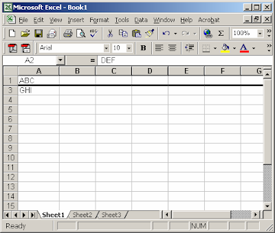
Answer: Select the entire row that you wish to hide.
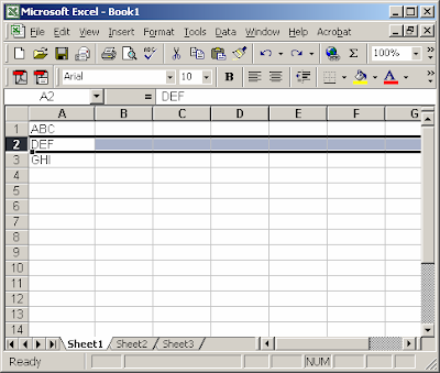
Right-click and select "Hide" from the popup menu.Your row should now be hidden.

Hide a row in Excel 2007

Also Learn how to Hide a row in Excel 2003/XP/2000/97

Question: How do I hide a row from being displayed in Excel 2007?

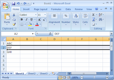
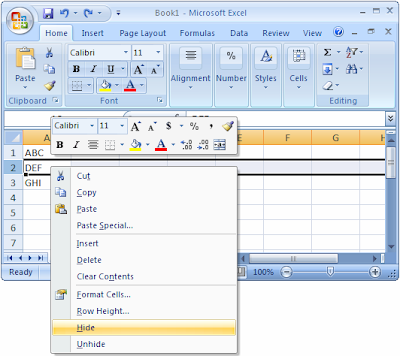
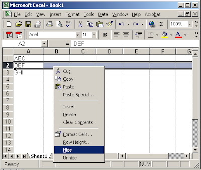
Answer: Select the entire row that you wish to hide.

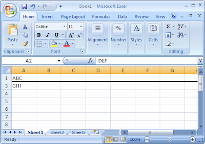
Right-click and select "Hide" from the popup menu.Your row should now be hidden.

Excel Topics: Rows

Hide / UnHide
Hide a Row in Excel 2007/Excel 2003/XP/2000/97
UnHide a row in Excel 2007/ Excel 2003/XP/2000/97
UnHide row 1 in Excel 2007/Excle 2003/XP/2000/97

Insert / Delete:
Insert a New Row in Excel 2007/ Excel 2003/XP/2000/97
Delete a Row in Excel 2007/Excle 2003/XP/2000/97

Sizing :
Change the height of a row in Excel 2007/ Excel 2003/XP/2000/97
Stop Wrap Text when pasting in Excel 2007/Excle 2003/XP/2000/97

Condition Formatting:
Automatically alrernate Row colors (One shaded, one white) in Excel 2007/Excle 2003/XP/2000/97
Automatically alternate row colors (Two shaded, tow white) in Excel 2007/ Excel 2003/XP/2000/97
Automatically alternate row colors (three shaded, three white ) in Excel 2007/Excle 2003/XP/2000/97

Create a column that must contain unique values in Excel 2003/XP/2000/97

Question: I'm looking for tips which can help me in creating a data column (Alphanumeric) in Excel 2003/XP/2000/97 where each row has to hold unique data. If a user enters a duplicate value in the column, the spreadsheet should not accept this value.

Answer: There are several "events" available within an Excel spreadsheet where you can place VBA code. In your case, we want to check for a duplicate value when the "Worksheet_Change" event fires.

Let's take a look at an example.
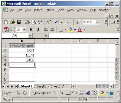
In our spreadsheet, we've set up column A in Sheet1 to contain unique values. On this sheet, we've placed code on the "Worksheet_Change" event, so that whenever a value is entered in column A (within the first 200 rows), the macro will test to see if this value has been entered before.

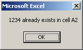
If the value is a duplicate, the following message will appear:

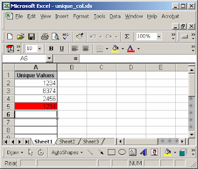
And the background color of the cell that contains the duplication will turn red.

In this example, we've entered the value 1234 in cell A5 which already exists in cell A2.

You can press Alt-F11 to view the VBA code.



Macro Code:
The macro code looks like this:

Private Sub Worksheet_Change(ByVal Target As Excel.Range)

Dim LLoop As Integer
Dim LTestLoop As Integer

Dim Lrows As Integer
Dim LRange As String
Dim LChangedValue As String
Dim LTestValue As String

'Test first 200 rows in spreadsheet for uniqueness
Lrows = 200
LLoop = 2

'Check first 200 rows in spreadsheet
While LLoop <= Lrows
LChangedValue = "A" & CStr(LLoop)

If Not Intersect(Range(LChangedValue), Target) Is Nothing Then
If Len(Range(LChangedValue).Value) > 0 Then

'Test each value for uniqueness
LTestLoop = 2
While LTestLoop <= Lrows
If LLoop <> LTestLoop Then
LTestValue = "A" & CStr(LTestLoop)
'Value has been duplicated in another cell
If Range(LChangedValue).Value = Range(LTestValue).Value Then
'Set the background color to red
Range(LChangedValue).Interior.ColorIndex = 3
MsgBox Range(LChangedValue).Value & " already exists in cell A" & LTestLoop
Exit Sub
Else
Range(LChangedValue).Interior.ColorIndex = xlNone
End If

End If

LTestLoop = LTestLoop + 1
Wend

End If
End If

LLoop = LLoop + 1
Wend

End Sub

Test for duplicates in eight columns, combined (and clear the values in the 8 columns when a duplicate is found) in Excel 2003/XP/2000/97

Question: In Excel 2003/XP/2000/97, is it possible to write a macro to check 8 columns over 2000 rows and clear the values in the 8 columns when a duplicate is found?

Answer: Let's take a look at an example.

In our spreadsheet, we've set up values in columns A through I. On Sheet1, we've created a button that when clicked will launch a macro. This macro will clear the values in columns A through H when a duplicate is found (based on the values in columns A through H). It does not clear the value in column I when a duplicate is found.

When the macro has completed, a message box will appear that indicates how many duplicates were cleared..

After the macro has run, you can see that cells A through H of the duplicate have been cleared, as seen below in rows 9 and 16.

You can press Alt-F11 to view the VBA code.

Please note that the LRows variable in this macro is set to 2000 indicating that the macro will test the first 2000 rows in for duplicates. You may need to change this value to accommodate your volume of data.



Macro Code:
The macro code looks like this:

Sub TestForDups()

Dim LLoop As Integer
Dim LTestLoop As Integer

Dim Lrows As Integer
Dim LRange As String

Dim LCnt As Integer

'Column values
Dim LColA_1, LColB_1, LColC_1, LColD_1, LColE_1, LColF_1, LColG_1, LColH_1 As String
Dim LColA_2, LColB_2, LColC_2, LColD_2, LColE_2, LColF_2, LColG_2, LColH_2 As String

'Test first 2000 rows in spreadsheet for duplicates (clear any duplicates found)
Lrows = 2000
LLoop = 2
LCnt = 0

'Check first 2000 rows in spreadsheet
While LLoop <= Lrows
LColA_1 = "A" & CStr(LLoop)
LColB_1 = "B" & CStr(LLoop)
LColC_1 = "C" & CStr(LLoop)
LColD_1 = "D" & CStr(LLoop)
LColE_1 = "E" & CStr(LLoop)
LColF_1 = "F" & CStr(LLoop)
LColG_1 = "G" & CStr(LLoop)
LColH_1 = "H" & CStr(LLoop)

If Len(Range(LColA_1).Value) > 0 Then

'Test each value for uniqueness
LTestLoop = LLoop + 1
While LTestLoop <= Lrows
If LLoop <> LTestLoop Then
LColA_2 = "A" & CStr(LTestLoop)
LColB_2 = "B" & CStr(LTestLoop)
LColC_2 = "C" & CStr(LTestLoop)
LColD_2 = "D" & CStr(LTestLoop)
LColE_2 = "E" & CStr(LTestLoop)
LColF_2 = "F" & CStr(LTestLoop)
LColG_2 = "G" & CStr(LTestLoop)
LColH_2 = "H" & CStr(LTestLoop)

'Value has been duplicated in another cell (based on values in columns A to H)
If (Range(LColA_1).Value = Range(LColA_2).Value) _
And (Range(LColB_1).Value = Range(LColB_2).Value) _
And (Range(LColC_1).Value = Range(LColC_2).Value) _
And (Range(LColD_1).Value = Range(LColD_2).Value) _
And (Range(LColE_1).Value = Range(LColE_2).Value) _
And (Range(LColF_1).Value = Range(LColF_2).Value) _
And (Range(LColG_1).Value = Range(LColG_2).Value) _
And (Range(LColH_1).Value = Range(LColH_2).Value) Then

'Clear the duplicate
Range("A" & CStr(LTestLoop) & ":H" & CStr(LTestLoop)).Select
Selection.ClearContents

LCnt = LCnt + 1

End If

End If

LTestLoop = LTestLoop + 1
Wend

End If

LLoop = LLoop + 1
Wend

'Reposition back on cell A1
Range("A1").Select
MsgBox CStr(LCnt) & " rows have been cleared."

End Sub

Test for duplicates in eight columns, combined (and delete duplicates and originals that were duplicated) in Excel 2003/XP/2000/97

Question: In Excel 2003/XP/2000/97, is it possible to write a macro to check 8 columns over 2000 rows and delete the duplicates as well as the original row that the duplicate was based on?

Answer: Let's take a look at an example.
In our spreadsheet, we've set up values in columns A through H. On Sheet1, we've created a button that when clicked will launch a macro. This macro will delete any duplicate values as well as the original row that the duplicate was based on (based on the values in columns A through H).

When the macro has completed, a message box will appear that indicates how many duplicate rows were deleted.

After the macro has run, you can see that four rows have been deleted.

You can press Alt-F11 to view the VBA code.

Please note that the LRows variable in this macro is set to 2000 indicating that the macro will test the first 2000 rows in for duplicates. You may need to change this value to accommodate your volume of data.



Macro Code:
The macro code looks like this:

Sub TestForDups()

Dim LLoop As Integer
Dim LTestLoop As Integer

Dim Lrows As Integer
Dim LRange As String

Dim LCnt As Integer

'Column values
Dim LColA_1, LColB_1, LColC_1, LColD_1, LColE_1, LColF_1, LColG_1, LColH_1, LColI_1 As String
Dim LColA_2, LColB_2, LColC_2, LColD_2, LColE_2, LColF_2, LColG_2, LColH_2, LColI_2 As String

'Test first 2000 rows in spreadsheet for duplicates (delete any duplicates found as well
' as the original row)
Lrows = 2000
LLoop = 2

'First pass: Check first 2000 rows in spreadsheet (only flag records for deletion)
While LLoop <= Lrows
LColA_1 = "A" & CStr(LLoop)
LColB_1 = "B" & CStr(LLoop)
LColC_1 = "C" & CStr(LLoop)
LColD_1 = "D" & CStr(LLoop)
LColE_1 = "E" & CStr(LLoop)
LColF_1 = "F" & CStr(LLoop)
LColG_1 = "G" & CStr(LLoop)
LColH_1 = "H" & CStr(LLoop)
LColI_1 = "I" & CStr(LLoop)

If Len(Range(LColA_1).Value) > 0 Then

'Test each value for uniqueness
LTestLoop = LLoop + 1
While LTestLoop <= Lrows
If LLoop <> LTestLoop Then
LColA_2 = "A" & CStr(LTestLoop)
LColB_2 = "B" & CStr(LTestLoop)
LColC_2 = "C" & CStr(LTestLoop)
LColD_2 = "D" & CStr(LTestLoop)
LColE_2 = "E" & CStr(LTestLoop)
LColF_2 = "F" & CStr(LTestLoop)
LColG_2 = "G" & CStr(LTestLoop)
LColH_2 = "H" & CStr(LTestLoop)
LColI_2 = "I" & CStr(LTestLoop)

'Value has been duplicated in another cell (based on values in columns A to H)
If (Range(LColA_1).Value = Range(LColA_2).Value) _
And (Range(LColB_1).Value = Range(LColB_2).Value) _
And (Range(LColC_1).Value = Range(LColC_2).Value) _
And (Range(LColD_1).Value = Range(LColD_2).Value) _
And (Range(LColE_1).Value = Range(LColE_2).Value) _
And (Range(LColF_1).Value = Range(LColF_2).Value) _
And (Range(LColG_1).Value = Range(LColG_2).Value) _
And (Range(LColH_1).Value = Range(LColH_2).Value) Then

'Flag the duplicate and original for deletion
Range(LColI_1).Value = "DELETE"
Range(LColI_2).Value = "DELETE"

End If
End If

LTestLoop = LTestLoop + 1
Wend

End If

LLoop = LLoop + 1
Wend

LCnt = 0
LLoop = 2

'Second pass: Delete records flagged for deletion
While LLoop <= Lrows
If Range("I" & CStr(LLoop)) = "DELETE" Then

'Delete row
Rows(CStr(LLoop) & ":" & CStr(LLoop)).Select
Selection.Delete Shift:=xlUp

'Decrement counter since row was deleted
LLoop = LLoop - 1

LCnt = LCnt + 1

End If

LLoop = LLoop + 1
Wend

'Reposition back on cell A1
Range("A1").Select
MsgBox CStr(LCnt) & " rows have been deleted."

End Sub

Test for duplicates in eight columns, combined (and delete duplicates) in Excel 2003/XP/2000/97

Question: In Excel 2003/XP/2000/97, is it possible to write a macro to check 8 columns over 2000 rows and delete the duplicates?

Answer: Let's take a look at an example.
In our spreadsheet, we've set up values in columns A through H. On Sheet1, we've created a button that when clicked will launch a macro. This macro will delete any duplicate values (based on the values in columns A through H).

When the macro has completed, a message box will appear that indicates how many duplicate rows were deleted.

After the macro has run, you can see that two rows have been deleted.

You can press Alt-F11 to view the VBA code.

Please note that the LRows variable in this macro is set to 2000 indicating that the macro will test the first 2000 rows in for duplicates. You may need to change this value to accommodate your volume of data.



Macro Code:
The macro code looks like this:

Sub TestForDups()

Dim LLoop As Integer
Dim LTestLoop As Integer

Dim Lrows As Integer
Dim LRange As String

Dim LCnt As Integer

'Column values
Dim LColA_1, LColB_1, LColC_1, LColD_1, LColE_1, LColF_1, LColG_1, LColH_1 As String
Dim LColA_2, LColB_2, LColC_2, LColD_2, LColE_2, LColF_2, LColG_2, LColH_2 As String

'Test first 2000 rows in spreadsheet for duplicates (delete any duplicates found)
Lrows = 2000
LLoop = 2
LCnt = 0

'Check first 2000 rows in spreadsheet
While LLoop <= Lrows
LColA_1 = "A" & CStr(LLoop)
LColB_1 = "B" & CStr(LLoop)
LColC_1 = "C" & CStr(LLoop)
LColD_1 = "D" & CStr(LLoop)
LColE_1 = "E" & CStr(LLoop)
LColF_1 = "F" & CStr(LLoop)
LColG_1 = "G" & CStr(LLoop)
LColH_1 = "H" & CStr(LLoop)

If Len(Range(LColA_1).Value) > 0 Then

'Test each value for uniqueness
LTestLoop = LLoop + 1
While LTestLoop <= Lrows
If LLoop <> LTestLoop Then
LColA_2 = "A" & CStr(LTestLoop)
LColB_2 = "B" & CStr(LTestLoop)
LColC_2 = "C" & CStr(LTestLoop)
LColD_2 = "D" & CStr(LTestLoop)
LColE_2 = "E" & CStr(LTestLoop)
LColF_2 = "F" & CStr(LTestLoop)
LColG_2 = "G" & CStr(LTestLoop)
LColH_2 = "H" & CStr(LTestLoop)

'Value has been duplicated in another cell (based on values in columns A to H)
If (Range(LColA_1).Value = Range(LColA_2).Value) _
And (Range(LColB_1).Value = Range(LColB_2).Value) _
And (Range(LColC_1).Value = Range(LColC_2).Value) _
And (Range(LColD_1).Value = Range(LColD_2).Value) _
And (Range(LColE_1).Value = Range(LColE_2).Value) _
And (Range(LColF_1).Value = Range(LColF_2).Value) _
And (Range(LColG_1).Value = Range(LColG_2).Value) _
And (Range(LColH_1).Value = Range(LColH_2).Value) Then

'Delete the duplicate
Rows(CStr(LTestLoop) & ":" & CStr(LTestLoop)).Select
Selection.Delete Shift:=xlUp

'Decrement counter since row was deleted
LTestLoop = LTestLoop - 1

LCnt = LCnt + 1

End If

End If

LTestLoop = LTestLoop + 1
Wend

End If

LLoop = LLoop + 1
Wend

'Reposition back on cell A1
Range("A1").Select
MsgBox CStr(LCnt) & " rows have been deleted."

End Sub

Test for duplicates in two columns, combined in Excel 2003/XP/2000/97

Question: In Excel 2003/XP/2000/97, is it possible to write a macro which would highlight any duplicate values where both columns A and B in two or more lines are the same?

Answer: Let's take a look at an example.
In our spreadsheet, we've set up values in both columns A and B. On this sheet, we've created a button that when clicked will launch a macro. This macro will highlight any duplicate values where both columns A and B in two or more lines are the same.

In our example, we've clicked on the button. Now the background color of the duplicates will turn red as follows:

In this example, the same values have been entered in rows 2 and 6.

You can press Alt-F11 to view the VBA code.

Please note that the LRows variable in this macro is set to 200 indicating that the macro will test the first 200 rows in columns A and B for duplicates. You may need to change this value to accommodate your volume of data.



Macro Code:
The macro code looks like this:

Sub TestForDups()

Dim LLoop As Integer
Dim LTestLoop As Integer
Dim LClearRange As String

Dim Lrows As Integer
Dim LRange As String

'Column A values
Dim LChangedValue As String
Dim LTestValue As String

'Column B values
Dim LChangedValueB As String
Dim LTestValueB As String

'Test first 200 rows in spreadsheet for uniqueness
Lrows = 200
LLoop = 2

'Clear all flags
LClearRange = "A2:B" & Lrows
Range(LClearRange).Interior.ColorIndex = xlNone

'Check first 200 rows in spreadsheet
While LLoop <= Lrows
LChangedValue = "A" & CStr(LLoop)
LChangedValueB = "B" & CStr(LLoop)

If Len(Range(LChangedValue).Value) > 0 Then

'Test each value for uniqueness
LTestLoop = 2
While LTestLoop <= Lrows
If LLoop <> LTestLoop Then
LTestValue = "A" & CStr(LTestLoop)
LTestValueB = "B" & CStr(LTestLoop)
'Value has been duplicated in another cell
If (Range(LChangedValue).Value = Range(LTestValue).Value) And (Range(LChangedValueB).Value = Range(LTestValueB).Value) Then
'Set the background color to red in column A
Range(LChangedValue).Interior.ColorIndex = 3
Range(LTestValue).Interior.ColorIndex = 3

'Set the background color to red in column B
Range(LChangedValueB).Interior.ColorIndex = 3
Range(LTestValueB).Interior.ColorIndex = 3

End If

End If

LTestLoop = LTestLoop + 1
Wend

End If

LLoop = LLoop + 1
Wend

End Sub

Test for duplicates on partial cell contents in a column in Excel 2003/XP/2000/97

Question: In Excel 2003/XP/2000/97, is it possible to write a macro which would highlight any duplicate values in column A? My problem is that sometimes the cell values do not match exactly.

For example, cell A1 contains "1234" and cell A2 contains "1234, 5678". Is there a way to compare partial cell contents so that a duplicate entry flag would be set for cells A1 and A2 in this example?

Answer: Let's take a look at an example.

In our spreadsheet, we've set up column A to contain unique values. On this sheet, we've created a button that when clicked will launch a macro. This macro will highlight any duplicate values in column A.

In our example, we've clicked on the button. Now the background color of the partial duplicates will turn red as follows:

In this example, the partial value of 1234 has been entered in cells A2, A5, and A6.

You can press Alt-F11 to view the VBA code.

Please note that the LRows variable in this macro is set to 200 indicating that the macro will test the first 200 rows in column A for duplicates. You may need to change this value to accommodate your volume of data.



Macro Code:
The macro code looks like this:

Sub TestForDups()

Dim LLoop As Integer
Dim LTestLoop As Integer
Dim LClearRange As String

Dim Lrows As Integer
Dim LRange As String
Dim LChangedValue As String
Dim LTestValue As String

'Test first 200 rows in spreadsheet for uniqueness
Lrows = 200
LLoop = 2

'Clear all flags
LClearRange = "A2:A" & Lrows
Range(LClearRange).Interior.ColorIndex = xlNone

'Check first 200 rows in spreadsheet
While LLoop <= Lrows
LChangedValue = "A" & CStr(LLoop)

If Len(Range(LChangedValue).Value) > 0 Then

'Test each value for uniqueness
LTestLoop = 2
While LTestLoop <= Lrows
If LLoop <> LTestLoop Then
LTestValue = "A" & CStr(LTestLoop)
'Value has been duplicated in another cell
If InStr(Range(LTestValue).Value, Range(LChangedValue).Value) > 0 Then
'Set the background color to red
Range(LChangedValue).Interior.ColorIndex = 3
Range(LTestValue).Interior.ColorIndex = 3

End If

End If

LTestLoop = LTestLoop + 1

Wend

End If

LLoop = LLoop + 1
Wend

End Sub

Test for duplicates in a column in Excel 2003/XP/2000/97

Question: In Excel 2003/XP/2000/97, is it possible to write a macro which would highlight any duplicate values in column A?
Answer: Let's take a look at an example.

In our spreadsheet, we've set up column A to contain unique values. On this sheet, we've created a button that when clicked will launch a macro. This macro will highlight any duplicate values in column A.

In our example, we've clicked on the button. Now the background color of the duplicates will turn red as follows:

In this example, the same value has been entered in both cells A2 and A5.

You can press Alt-F11 to view the VBA code.

Please note that the LRows variable in this macro is set to 200 indicating that the macro will test the first 200 rows in column A for duplicates. You may need to change this value to accommodate your volume of data.

Macro Code:
The macro code looks like this:

Sub TestForDups()

Dim LLoop As Integer
Dim LTestLoop As Integer
Dim LClearRange As String

Dim Lrows As Integer
Dim LRange As String
Dim LChangedValue As String
Dim LTestValue As String

'Test first 200 rows in spreadsheet for uniqueness
Lrows = 200
LLoop = 2

'Clear all flags
LClearRange = "A2:A" & Lrows
Range(LClearRange).Interior.ColorIndex = xlNone

'Check first 200 rows in spreadsheet
While LLoop <= Lrows LChangedValue = "A" & CStr(LLoop) If Len(Range(LChangedValue).Value) > 0 Then

'Test each value for uniqueness
LTestLoop = 2
While LTestLoop <= Lrows If LLoop <> LTestLoop Then
LTestValue = "A" & CStr(LTestLoop)
'Value has been duplicated in another cell
If Range(LChangedValue).Value = Range(LTestValue).Value Then
'Set the background color to red
Range(LChangedValue).Interior.ColorIndex = 3
Range(LTestValue).Interior.ColorIndex = 3

End If

End If

LTestLoop = LTestLoop + 1

Wend

End If

LLoop = LLoop + 1
Wend

End Sub

Link data to a combo box and update underlying data in Excel 2003/XP/2000/97

Question: In Excel 2003/XP/2000/97, I want to be able to use a combo box (on another sheet) to display data from Sheet1 and then be able to edit that data and save the changes back to Sheet1. How can I do this?

Answer: This can be done with macro code.

Let's take a look at an example.

In our spreadsheet, our data is on Sheet1.

On Sheet2, we have our combo box which is linked to the data on Sheet1. When the user selects a customer in the combo box, the address and phone number will be automatically populated. The population of this data is done by a macro called PopulateData (which is the macro assigned to the combo box).

A user can then update the data on this sheet. In our example, we've changed Betty's address from 454 11th to 78 Granite St.

Next, we click on the Save Changes button. This calls a macro called SaveChanges.

The macro will update the corresponding data on Sheet1 and display the message above when it has completed.

Now if we go to Sheet1, we can see that the address for Betty has been updated.

You can press Alt-F11 to view the VBA code. Select the module called Module1 in the left window.

Macro Code

The macro code looks like this:

The macro code for the Save Changes button:

Sub SaveChanges()

'Update data on Sheet1 based on changes made to data on Sheet2

Dim LProject As Integer

Dim LAddress As String
Dim LPhoneNbr As String

Dim LRow As Long
Dim LFound As Boolean

'Retrieve project number number
LProject = Range("H3").Value

'Retrieve new address and phone number information
LAddress = Range("E5").Value
LPhoneNbr = Range("H8").Value

'Move to Sheet1 to save the changes
Sheets("Sheet1").Select

LFound = False

LRow = 2

Do While LFound = False

'Found matching project, now update address and phone number information

If Range("A" & LRow).Value = LProject Then
LFound = True
Range("C" & LRow).Value = LAddress
Range("D" & LRow).Value = LPhoneNbr

'Encountered a blank project number (assuming end of list on Sheet1)
ElseIf IsEmpty(Range("A" & LRow).Value) = True Then

MsgBox ("No match was found. Changes were not made.")
Exit Sub
End If

LRow = LRow + 1
Loop

'Reposition back on Sheet2
Sheets("Sheet2").Select
Range("E5").Select

MsgBox ("Changes were successfully saved.")

End Sub

The macro code for the customer combo box:

Sub PopulateData()

Dim LProject As Integer

Dim LAddress As String

Dim LPhoneNbr As String

Dim LRow As Long

Dim LFound As Boolean

'Retrieve project number number

LProject = Range("H3").Value

'Move to Sheet1
Sheets("Sheet1").Select

LFound = False

LRow = 2

Do While LFound = False
'Found matching project, now update address and phone number information on Sheet2

If Range("A" & LRow).Value = LProject Then

LFound = True

LAddress = Range("C" & LRow).Value

LPhoneNbr = Range("D" & LRow).Value

Sheets("Sheet2").Select
Range("E5").Value = LAddress
Range("H8").Value = LPhoneNbr

'Encountered a blank project number (assuming end of list on Sheet1)

ElseIf IsEmpty(Range("A" & LRow).Value) = True Then

MsgBox ("No match was found for combo box selection.")

Exit Sub

End If

LRow = LRow + 1
Loop

End Sub

Update a cell when a checkbox is clicked (Control Toolbox toolbar) in Excel 2003/XP/2000/97

Question:  In Excel 2003/XP/2000/97, is there a way to link a check box to another cell? For example, I've made a checkbox and whenever the checkbox is clicked, I would like the current date to automatically appear in another cell. Is this possible?

Also I would like the date to not change whenever the worksheet is opened. For example, if a cell has been set to July 16th and the worksheet is opened on July 17th, I still want the cell to read as July 16th.

Answer:  Because you don't want the cell value changing whenever the spreadsheet "recalculates", we'll have to create a macro to determine when to update the cell value.

Let's take a look at an example.

In our spreadsheet, there are two columns - column A contains a checkbox and column B contains the "linked" cell.

We've created various checkboxes in column A using the Control Toolbox toolbar. To view the Control Toolbox toolbar, select Toolbars > Control Toolbox under the View menu.

When the checkbox in column A is "checked", the associated cell in column B will be updated with the current system date. When the checkbox is "unchecked", the associated cell value will be cleared.

This is accomplished with a macro called Process_Checkbox. You can view the macro by pressing Alt-F11.

The macro determines what row the checkbox resides in and then "sets the value" of the associated cell in column B.

Macro Code:

The macro code looks like this:

Sub Process_CheckBox(pObject)

    Dim LRow As Integer

    Dim LRange As String

    'Find row that checkbox resides in

    LRow = pObject.TopLeftCell.Row

    LRange = "B" & CStr(LRow)

    'Change date in column B, if checkbox is checked


    If pObject.Value = True Then

        ActiveSheet.Range(LRange).Value = Date

    'Clear date in column B, if checkbox is unchecked

    Else

        ActiveSheet.Range(LRange).Value = Null

    End If

End Sub

Private Sub CheckBox1_Click()

    Process_CheckBox CheckBox1

End Sub

Private Sub CheckBox2_Click()


    Process_CheckBox CheckBox2

End Sub

Private Sub CheckBox3_Click()

    Process_CheckBox CheckBox3

End Sub

Private Sub CheckBox4_Click()


    Process_CheckBox CheckBox4

End Sub

Private Sub CheckBox5_Click()

    Process_CheckBox CheckBox5

End Sub

Private Sub CheckBox6_Click()


    Process_CheckBox CheckBox6

End Sub

Private Sub CheckBox7_Click()

    Process_CheckBox CheckBox7

End Sub

Update a cell when a checkbox is clicked (Forms toolbar) in Excel 2003/XP/2000/97

Question:  In Excel 2003/XP/2000/97, is there a way to link a check box to another cell? For example, I've made a checkbox and whenever the checkbox is clicked, I would like the current date to automatically appear in another cell. Is this possible?

Also I would like the date to not change whenever the worksheet is opened. For example, if a cell has been set to July 16th and the worksheet is opened on July 17th, I still want the cell to read as July 16th.

Answer:  Because you don't want the cell value changing whenever the spreadsheet "recalculates", we'll have to create a macro to determine when to update the cell value.

Let's take a look at an example.

In our spreadsheet, there are two columns - column A contains a checkbox and column B contains the "linked" cell.

We've created various checkboxes in column A using the Forms toolbar. To view the Forms toolbar, select Toolbars > Forms under the View menu.

When the checkbox in column A is "checked", the associated cell in column B will be updated with the current system date. When the checkbox is "unchecked", the associated cell value will be cleared.

This is accomplished with a macro called Process_Checkbox. You can view the macro by pressing Alt-F11.

The macro determines what row the checkbox resides in and then "sets the value" of the associated cell in column B.

Macro Code:

The macro code looks like this:

Sub Process_CheckBox()

    Dim cBox As CheckBox

    Dim LRow As Integer


    Dim LRange As String

    LName = Application.Caller

    Set cBox = ActiveSheet.CheckBoxes(LName)

    'Find row that checkbox resides in

    LRow = cBox.TopLeftCell.Row


    LRange = "B" & CStr(LRow)

    'Change date in column B, if checkbox is checked

    If cBox.Value > 0 Then

        ActiveSheet.Range(LRange).Value = Date

    'Clear date in column B, if checkbox is unchecked

    Else

        ActiveSheet.Range(LRange).Value = Null

    End If

End Sub

Update cell based on hyperlink selected

Question: I have created a hyperlink from one worksheet to another within the same file. But when the linked worksheet is pulled up, I want to populate the designated field with some text. The text will change depending on the hyperlink selected, but all the links will connect to the same worksheet and the same field. The field I am wanting to populate controls numerous lookup functions.

HELP!! Can this be done?

Answer: Yes, this can be done by utilizing macros on two Excel workbook "events".

Let's take a look at an example.

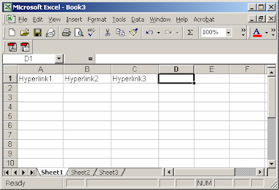
In our spreadsheet, there are two sheets called Hyperlinks and Destination. The Hyperlinks sheet contains three hyperlinks in cell A3, A6, and A9. All three hyperlinks point to cell B2 in the Destination sheet

When a hyperlink is clicked, the Destination sheet is activated and cell B2 will display text showing which hyperlink was selected. In our example below, we've selected "Hyperlink #1" in cell A3.

You can view the macros by pressing Alt-F11 and double-clicking on the ThisWorkbook object in the left window.

There are three components to this solution:

1. There is a global variable called GSourceCell which contains the cell reference when the hyperlink was selected.


2. There is a workbook event called "SheetSelectionChanged". When this event fires, the GSourceCell variable will be populated


3. There is a workbook event called "SheetFollowHyperlink". When this event fires, cell B2 in the Destination sheet will be populated with text.

Macro Code:

The macro code looks like this:

Private Sub Workbook_SheetFollowHyperlink(ByVal Sh As Object, ByVal Target As Hyperlink)

'Update cell B2 in Destination sheet based on the origin of hyperlink
If Sh.Name = "Hyperlinks" Then
If GSourceCell = "A3" Then
Sheets("Destination").Range("B2").Value = "Hyperlinked from cell A3"
ElseIf GSourceCell = "A6" Then
Sheets("Destination").Range("B2").Value = "Hyperlinked from cell A6"
ElseIf GSourceCell = "A9" Then
Sheets("Destination").Range("B2").Value = "Hyperlinked from cell A9"
Else
Sheets("Destination").Range("B2").Value = ""
End If
End If

End Sub

Private Sub Workbook_SheetSelectionChange(ByVal Sh As Object, ByVal Target As Range)

If Sh.Name = "Hyperlinks" Then
'Capture last active cell on Hyperlinks worksheet and store in global variable
GSourceCell = Target.Address(False, False)
End If

End Sub

Delete all hyperlinks on a sheet in Excel 2003/XP/2000/97

Question: I've had a hyperlink problem in my Excel files for ages: false hyperlinks had crept in (even in empty cells) and were multiplying regularly whenever I inserted new lines. How can I delete all hyperlinks in a sheet at once and not have to delete them cell by cell?

Answer: You will need to create a macro to delete the hyperlink addresses in your Excel sheet.

Open your Excel spreadsheet that you wish to remove the hyperlinks from. Press -F11 to go to the Visual Basic editor. Create a new module. You can do this by selecting Module under the Insert menu.

Paste the following code into your new module:

Sub RemoveHyperlinks()

'Remove all hyperlinks from the active sheet
ActiveSheet.Hyperlinks.Delete

End Sub

Close the Visual Basic editor window by selecting "Close and Return to Microsoft Excel" under the File menu.

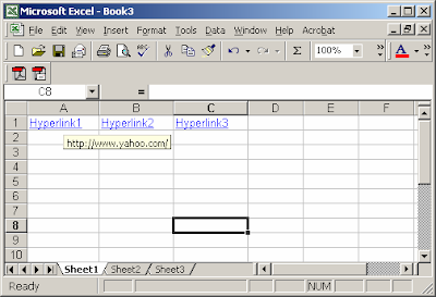
Now, go to the sheet that contains the hyperlinks that you wish to delete. Here is an example of a sheet with multiple hyperlink addresses:

Under the Tools menu, select Macro > Macros. Highlight the macro called "RemoveHyperlinks" and click on the Run button.

Now your hyperlinks should be deleted as you can see by the example below:

If you need to remove hyperlinks from other sheets, just repeat the steps above.

Filter final series of numbers in hyperlink address in Excel 2003/XP/2000/97

Question: I've downloaded a table from the web with hyperlink references into Excel 2003/XP/2000/97. I need to filter out the final series of numbers for each hyperlink address and put them as a number in a column. How can I do this?

Answer: Below is a function that you can include in your spreadsheet to filter the final series of numbers in a hyperlink address in Excel.

Function FinalNumberSeries(pCell) As Long

Dim LChar As String
Dim LLength As Integer
Dim LStart As Integer
Dim LExit As Boolean

LLength = Len(pCell)
LStart = LLength
LExit = False

'Search backwards through the string until a non-numeric
'character is found
Do Until LExit = True
LChar = Mid(pCell, LStart, 1)

If IsNumeric(LChar) = False Then
LExit = True
ElseIf LStart = 1 Then
LExit = True
End If

LStart = LStart - 1
Loop

FinalNumberSeries = Mid(pCell, LStart + 2)

End Function

Then you can reference this new function in your spreadsheet.

For example in cell B1, you could enter the following:

=FinalNumberSeries(A1)

Excel: Extract hyperlink address (files and web addresses) in Excel 2003/XP/2000/97

Question: In Excel 2003/XP/2000/97, I have a spreadsheet that contains hyperlink addresses to files. I tried extracting the hyperlink address for these files, however I'm not getting the complete Address. The complete Address should be:

C:\My Documents\Past Projects\Centennial\Program Status Report.xls

But I only get:

\..\..\Past Projects\Centennial\Program Status Report.xls

Is there a way to always get the complete hyperlink address?

Answer: Below are two functions that you can include in your spreadsheet to extract the complete hyperlink address for either a file of a web address.

Function HyperLinkText(pRange As Range) As String

Dim ST1 As String
Dim ST2 As String
Dim LPath As String
Dim ST1Local As String
If pRange.Hyperlinks.Count = 0 Then
Exit Function
End If

LPath = ThisWorkbook.FullName
ST1 = pRange.Hyperlinks(1).Address
ST2 = pRange.Hyperlinks(1).SubAddress

If Mid(ST1, 1, 15) = "..\..\..\..\..\" Then
ST1Local = ReturnPath(LPath, 5) & Mid(ST1, 15)
ElseIf Mid(ST1, 1, 12) = "..\..\..\..\" Then
ST1Local = ReturnPath(LPath, 4) & Mid(ST1, 12)
ElseIf Mid(ST1, 1, 9) = "..\..\..\" Then
ST1Local = ReturnPath(LPath, 3) & Mid(ST1, 9)
ElseIf Mid(ST1, 1, 6) = "..\..\" Then
ST1Local = ReturnPath(LPath, 2) & Mid(ST1, 6)
ElseIf Mid(ST1, 1, 3) = "..\" Then
ST1Local = ReturnPath(LPath, 1) & Mid(ST1, 3)
Else
ST1Local = ST1
End If

If ST2 <> "" Then
ST1Local = "[" & ST1Local & "]" & ST2
End If

HyperLinkText = ST1Local

End Function

Function ReturnPath(pAppPath As String, pCount As Integer) As String

Dim LPos As Integer
Dim LTotal As Integer
Dim LLength As Integer

LTotal = 0
LLength = Len(pAppPath)

Do Until LTotal = pCount + 1
If Mid(pAppPath, LLength, 1) = "\" Then
LTotal = LTotal + 1
End If
LLength = LLength - 1
Loop

ReturnPath = Mid(pAppPath, 1, LLength)

End Function

Then you can reference these new functions in your spreadsheet.

For example in cell B1, you could enter the following:

=HyperLinkText(A1)

Extract Hyperlink address (Web addresses only) in Excel 2003/Xp/2000/97

Question : I've downloaded a table from the web with hyperlink references into Excel 2003/XP/2000/97. What I need to do is examine the hypertext link and extract a small part of that link. All I seem to get is the details of the link in a pop up box (yellow) and any attempt to filter out detail only results in the display of the destination ?

Is there a way I can examine a hyperlink details without invoking the hyperlink?


Answer: Below is a function that you can include in your spreadsheet to extract the hyperlink address from a cell in Excel.

Function HyperLinkText(pRange As Range) As String

Dim ST1 As String
Dim ST2 As String

If pRange.Hyperlinks.Count = 0 Then
Exit Function
End If

ST1 = pRange.Hyperlinks(1).Address
ST2 = pRange.Hyperlinks(1).SubAddress

If ST2 <> "" Then
ST1 = "[" & ST1 & "]" & ST2
End If

HyperLinkText = ST1

End Function

Then you can reference this new function in your spreadsheet.
For example in cell B1, you could enter the following:

=HyperLinkText(A1)

Excel Topics: Macros

Hyperlinks:
Extract hyperlink address (Web addresses only) in Excel 2003/Xp/2000/97

Extract hyperlink address (Files & Web addresses only) in Excel 2003/Xp/2000/97

Filter Final Series of numbers in hyperlink address in Excel 2003/XP/2000/97

Delete all hyperlinks on a sheet in Excel 2003/Xp/2000/97

Update cell based on hyperlink selected in Excel 2003/Xp/2000/97

Checkboxes :
Update a cell when a checkbox is clicked (Forms toolbar) in Excel 2003/Xp/200/97

Update a cell when a checkbox is clicked (Control ToolBox Toolbar) in Excel 2003/ Xp / 2000/97

Combo boxes:
Link data to combo box and update underlying data in Excel 2003/Xp/2000/97


Test for Duplicates :
Test for Duplicates in a column in Excel 2003/Xp/2000/97
Test for Duplicates on partial cell contents in a Column in Excel 2003/Xp/2000/97
Test for Duplicates in Two Columns, combined in Excel 2003/Xp/2000/97
Test for Duplicates in eight columns, combined (and delete duplicates) in Excel 2003/Xp/97
Test for Duplicates in Eight Columns, combined (And delete duplicates and originals that we duplicated ) in Excel 2003/Xp/ 2000/97
Test for duplicates in Eight columns, Combined ( & Clear the values in the 8 Columens when a duplicate is found) in Excel 2003/XP/2000/97
Create a column that must contain unique values in Excel 2003/XP/2000/97

Test & Copy Data :
Test each value in column A untill a diffrent value is found in Excel 2003/Xp/2000/97
Test each value in column A & copy matching values into new sheets in Excel 2003/XP/2000/97
Test each value in column A & copy matching values into new workbooks in Excel 2003/XP/2000/97.
Test each value in column A & copy matching values into new workbooks (name workbooks the value found in column A ) in Excel 2003/Xp/2000/97
Copy the value in Column B the number of times indicated by the value in Column A in Excel 2003/Xp/2000/97
Copy range of cells form one sheet to another sheet matching on date values in Excel 2003/XP/2000/97
Search for a value in a column and copy row to new sheet for all matching values in Excel 2003/XP/2000/97
Enter a value in an InputBox and then search for this value in a column and copy row to new sheet for all matching values in Excel 2003/XP/2000/97
Copy date to various sheets based on the value in column A in Excel 2003/XP/2000/97

Update Formulas :
Update all formulas to reference data in a particular column in Excel 2003/Xp/2000/97
Update all formulas to refrence data in a particular row in Excel 2003/Xp/2000/97

Integration with Access :
Open an Access Form form Excel 2003/Xp/2000/97

Custom Math Functions :
Creating a Custom round function in Excel 2003/Xp/2000/97
Creating a custom average function (that excludes outlyers form the calculation) in Excel 2003/Xp/2000/97

Check if Files Exist :
Check to see if a file exist based on a value in Column A in Excel 2003/Xp/2000/97
Check to see if files exist based on values form 2 Columns in Excel 2003/Xp/2000/97

Miscellaneous in Excel 2003/Xp/2000/97 :
Test Range of Cells for Formulas (or missing Formulas)
Automatically refresh Pivot Table when data in a sheet changes
Automatically refresh Pivot Table when user Switches between sheets
Link one cell to another cell (Control the recalculation)
Change the Background colour of a row based on a cell value
Change the Background colour of a cell when another cell is selected
Macro to warm when a recorrd will expire within 31 Days
Convert currency into words
Overwrite column B value when column A value is higher
Function to Calculate total cost based on a tiered fee structure
Autonumber a cell each time the Spreadsheet is opened
Convert an entire spreadsheet to proper case
Convert an entire spreadsheet to Uppercase
Convert custom function to exceed 7 nested If functions
Create a control screen to maintain data on another sheet
Counting matched pairs
Perform a lookup where the refrences value is stored somewhere in a string
Cleanup an export of raw data
Re-arrange data in an export of raw data
Create in a File Save as macro
Test a string for an alphanumeric value
Automatically open a Form when spreadsheet is opened
Count the number of cells with a particular font color

Excel: Draw a line through a value in a cell (strikethrough) in Excel 2003/XP/2000/97

Also Learn how to Draw a strikethrough in Excel 2007.
Question : How Do I Draw a line through a value in a cell in Excel 2003/XP/2000/97 ?
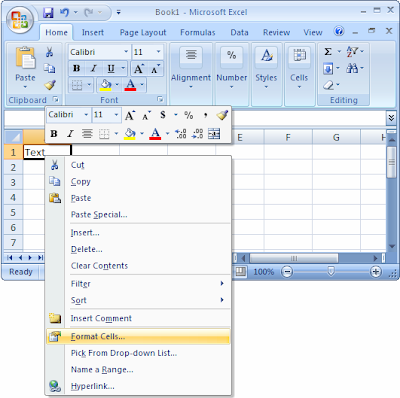
Answer : Select the Text that you wish to stikethrough. This can either be the entire cell or only a character in the cell. While your mouse is over the selected text, Right- Click and then select "Format Cells" From the popup menu.

When the Format Cells window appears, select the Font Tab. check the Strikethrough Checkbox. Click on the Ok Button.

Now When you retrun to your spreadsheet, you should see a strike throuhg your selected text.

Excel : Draw a line through a value in a cell (Strike through) in Excel 2007

Also Learn How to Draw a strickthrough in Excel 2003/XP/2000/97
Question : How do I draw a line through a value in a cell in Excel 2007 ?
Answer : Select the Text that you wish to Strikethrough. This can either be the Entire cell or only a character in the cell. While your mouse is over the selected text, Right - Click and then select " Fromat Cells " From the popup menu.

When the Format cells window appears, select the Font Tab. Check the Strikethought checkbox. Click on the OK Button.

Now when you return to you Spreadsheet, you will see a strike through your selected text.

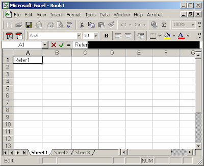
Excel : Create a subscript value in a cell in Excel 2003/XP2000/97

Also Learn how to create a subsctipt value in a cell in Excel 2007.
Question : How do I Create a subscript value in a cell in Excel 2003/Xp/2000/97 ?
Answer : Select text that you wish to convert to subscript. This can either be the entire cell or only a character in the cell.

While your mouse is over the Selected text, Right - Click and then select "Format Cells" From the popup menu.

When the Format Cells window appears, select the Font Tab. check the Subscript checkbox.

Now when you return to the spreadsheet, you should see the subscript value.

Excel: Create a Subscript Value in a cell in Excel 2007

Also Learn How to Create a Subscript value in a cell in Excel 2003/XP/2000/97
Question : How Do I Create a Subscript value in a cell in Excel 2007 ?
Answer : Select the Text that you wish to convert to subscript. This can either be the entire cell or only a character in the cell.

While your mouse is over the selected text, Right-Click and then select " Format Cells" From the popup menu.

When the Format Cells Window appears, select the Font Tab. Check the Subscript checkbox.

Now when you return to the spreadsheet, you should see the subscript value.